+ W& @" q [7 g; p' V2 _ 推荐一个超好用的python包folium, 专门用于地理数据可视化,官方英文教程教程点击这里。
; v0 ~ o/ S& d
, F& j3 O4 k8 ^! Q! t 使用方法很简单,操作如下:
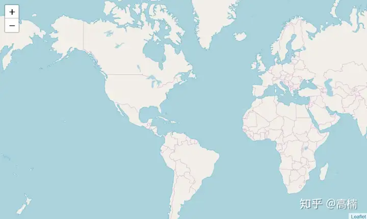
导入包,创建一副世界地图
, }: P' I5 g* V, O import folium" t) E* L, @4 f( D8 m8 o# w
import pandas as pd
' k. X# {+ {( P) w9 M' ]! v* H1 E$ F$ E% X7 ?! H
# define the world map
' K9 Y0 g9 g5 v! ]) ] world_map = folium.Map(); |3 |8 L# X, p/ V0 O, E' W
* y. k5 ^6 F. ]4 }: A w
# display world map2 p r' b. V2 v1 S% C' ?8 c( Z g) \2 n
world_map
$ r; h2 l+ } S- Q# M$ ~ * b1 n0 c* R! U% t# Z; g7 F
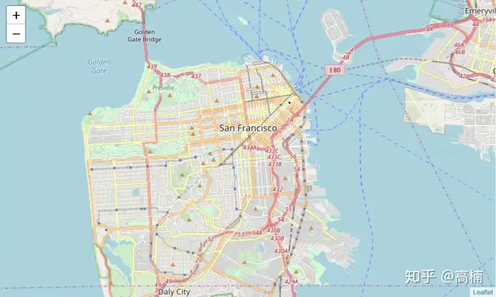
2. 输入经纬度,尺度,在这里我们以旧金山(37.7749° N, 122.4194° W)为例。
& v# m( ]+ K- b" X # San Francisco latitude and longitude values
: t8 k; O) P/ l, _ latitude = 37.77
) @; H9 h$ b' H7 C# O8 d6 z# j6 D4 Z longitude = -122.42
- q6 }% ^* I/ f5 r
* h- J7 k* ]; _ # Create map and display it
; _4 X1 o/ `/ N- c% p( V: f san_map = folium.Map(location=[latitude, longitude], zoom_start=12)
8 g. C. c8 p N2 X
* q3 c8 O1 @/ j) j0 {! K& r' ^ # Display the map of San Francisco
, a# d; }! q3 N3 ?' _# h san_map
2 Y& q' G H% Y# {, b$ k8 E
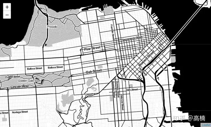
7 s& r5 v8 G' ?6 K$ `+ M5 {% t) c 更改地图显示,默认为OpenStreetMap风格,我们还可以选择Stamen Terrain, Stamen Toner等。
0 ^8 h9 C; J: s, K7 x
# Create map and display it7 H3 w1 U" \! n# Z& h3 N8 y; {
san_map = folium.Map(location=[latitude, longitude], zoom_start=12,tiles=Stamen Toner)
! \# _! F& z. j! @5 L6 F
) g1 F+ \* b8 h: E& K+ l; Y
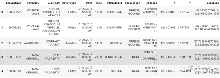
3. 读取数据集(旧金山犯罪数据集)
; S$ g3 x6 F8 `( B: n. ]0 p
# Read Dataset
* q2 {( e r, f% ]2 C9 l+ x cdata = pd.read_csv(https://cocl.us/sanfran_crime_dataset)- q) P. e. p% p
cdata.head()
" l& y- i# C) q
5 I8 s9 w2 T# f+ Y$ b4 S
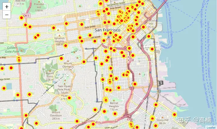
4. 在地图上显示前200条犯罪数据
# E: Y2 i8 A. ~- E9 Y # get the first 200 crimes in the cdata
3 \3 p; B% d, }# v
limit = 200
. E+ L9 h: Y% b z4 { J data = cdata.
iloc[0:limit, :]
/ |, a& Z0 \. v7 c
0 f5 J5 @# G$ _. E # Instantiate a feature group for the incidents in the dataframe
6 {# A$ b$ A6 O+ u
incidents = folium.map.FeatureGroup()
5 {5 ]$ N! h! r6 x* K& ]
6 M# A" @, ~% K4 M # Loop through the 200 crimes and add each to the incidents feature group
* O/ `6 z) z; ]( m. h for lat, lng, in zip(cdata.Y, data.X):
& K) S7 v9 i. T! T! e/ ~4 n incidents.add_child(
6 u- j8 L: l/ J1 q2 g5 ^ folium.CircleMarker(
' m2 H: {2 j8 H [lat, lng],
: I. F) G9 |5 Q9 n- \5 q/ C radius=7, # define how big you want the circle markers to be
' u! x# e4 n. \. k3 V# l
color=yellow,
4 U% I6 v' ^/ ]% F, B
fill=True,
" X! [# n1 P' k% e fill_color=red,
6 o/ b0 R/ n" i) o V8 t' U fill_opacity=0.4
# P- t5 V: y% m5 Q2 K# ^8 n )
8 \' T3 U: E3 R9 `% c )
$ Q8 [% F9 f$ x B: S6 Y4 G5 \
5 J4 A3 G. k. {2 S- s- U! h& T# G
# Add incidents to map
3 U6 |! K! e& ?8 q' B& i
san_map = folium.Map(location=[latitude, longitude], zoom_start=12)
3 {/ j: U* u8 R N# R$ }- H% r# H M# l
san_
map.add_child(incidents)
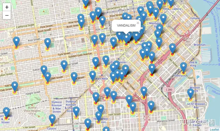
5. 添加地理标签
2 ?% k6 f6 Y% a) ~4 H
# add pop-up text to each marker on the map
& U' U2 f! C, N* w9 A ?
latitudes = list(data.Y)
) ^5 N6 c% C" S% I longitudes = list(data.X)
( Q$ ^1 |; l" J8 R, R* D labels = list(data.Category)
4 v; B& e( A! u4 t8 T: j6 h7 H% D7 L8 ]( t5 X' @+ o- Q0 g
for lat, lng, label in zip(latitudes, longitudes, labels):
& E" C& `+ m w s6 v/ S folium.Marker([lat, lng], popup=label).add_to(
san_map)
) e B+ @. h- k4 T* x6 j4 y2 x
9 J( P( }/ m$ U6 X$ j j+ j
# add incidents to map
& @0 E4 m) w$ ~$ @" P% L! ]& y, | san_map.add_child(incidents)
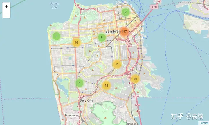
6. 统计区域犯罪总数
2 [4 U3 o' c3 ]8 \8 a6 X7 b! F from folium import plugins
9 b4 ?1 R, D+ q X& U
/ R( G1 k6 |# { d9 b9 @ # lets start again with a clean copy of the map of San Francisco
1 J3 n! y# j/ J$ c# k
san_map = folium.Map(location = [latitude, longitude], zoom_start = 12)
# e+ Z J8 K6 q5 p/ @
# g$ d; o& Z6 M* h$ t # instantiate a mark cluster object for the incidents in the dataframe
0 |1 \" x/ X2 F1 k: m incidents = plugins.MarkerCluster().add_to(san_map)
# `* X# l3 K* r& o
& d" U% k7 I0 i9 } # loop through the
dataframe and add each data point to the mark cluster
+ J& d4 [! L. T; S6 i Y for lat, lng, label, in zip(data.Y, data.X, cdata.Category):
9 u( S1 M4 M5 O) Y folium.Marker(
; Q' ~- e! L e
location=[lat, lng],
1 h$ t' h" R; y7 y0 u- ~, Y: I icon=None,
1 \: v; K+ I4 M/ Q8 D8 b* J7 c4 v
popup=label,
S$ b# s) e" c( c( D* | ).add_to(incidents)
! n6 ~! o4 M6 \5 y
7 e1 y9 u+ L9 o4 P8 b; t # add incidents to map
8 ]$ S& C" X0 x { san_map.add_child(incidents)
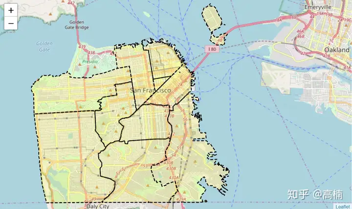
7. 读取geojson文件,可视化旧金山市10个不同Neighborhood的边界
0 l" i3 C& T" P) }2 w3 E import json/ M7 B+ K+ h5 S' H* _) y0 ~- G
import requests. q. J( R! N p
% X7 _+ y6 b8 k0 D5 y' M+ _1 I
url = https://cocl.us/sanfran_geojson' P( U3 _ X( v t- V3 K
san_geo = f{url}
# Z" H$ q7 B, f! m: |1 m. O" X7 D san_map = folium.Map(location=[37.77, -122.4], zoom_start=12)
6 F( Z+ V+ F( R, q$ I" v folium.GeoJson(* U+ n) D$ _1 A5 U2 l9 p& I) n
san_geo,
- d: c; Q5 p" y; K style_function=lambda feature: {/ S$ i6 q1 F( C9 l7 l/ F5 ^
fillColor: #ffff00,
) d( v* o4 |0 D/ ]' { color: black,2 T% ~# u! I/ G. a
weight: 2,
3 c8 J9 D* Z( s4 @ dashArray: 5, 5
* \ k% C9 L9 C" J }; \. ?1 R" k8 b/ n# p
).add_to(san_map)
2 n( H7 E: l( I4 j7 e. K: b6 z
6 a) Y6 C8 F; e3 }: w& n! X) C #display map+ {& _: a+ D1 c# o: U* x
san_map
+ P- z# a4 z3 N9 P( U0 E- f
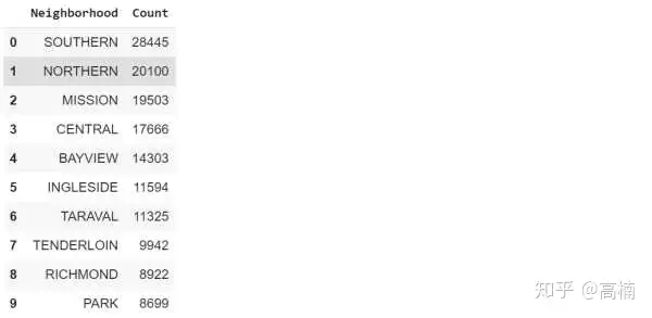
7 V+ h) S* D# S& n F) {+ R 8. 统计每个区域的犯罪事件数目
. {' K% D6 _" q' f; l% k4 ]6 D # Count crime numbers in each
neighborhood
. A. D0 e$ I, k/ V, U disdata = pd.DataFrame(cdata[PdDistrict].value_counts())
9 ?0 n5 V* A- R1 Z2 l% I. `" _5 X disdata.reset_index(inplace=True)
& `, h1 ~2 l3 W" x" ?/ N disdata.rename(columns={index:Neighborhood,PdDistrict:Count},inplace=True)
0 W- I" H0 R7 N$ k9 b- k% @" d) D$ z: d- n disdata
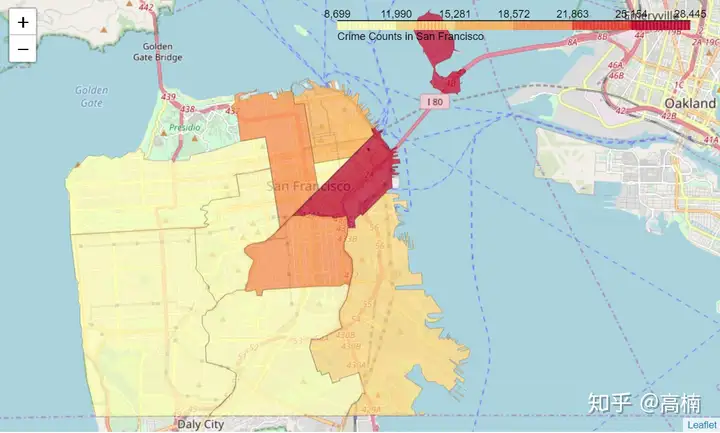
9. 创建Choropleth Map (颜色深浅代表各区犯罪事件数目)
/ ?, a0 z# E3 @7 ]/ a m = folium.Map(location=[37.77, -122.4], zoom_start=12)
5 S. v" g& o3 ]: C l
folium.Choropleth(
6 ?1 p# J, R; g2 I6 ]# F
geo_data=san_geo,
9 }% u1 t( `6 V9 I, H0 d1 E9 \ data=disdata,
( u: d8 z- E J* i; Z" } columns=[Neighborhood,Count],
& o0 w( S7 r/ U8 z- e; Y6 i9 l) j$ M
key_on=feature.properties.DISTRICT,
- T! \" Q4 f7 Y
#fill_color=red,
) b3 z% S. h/ |' W7 ^$ C7 j fill_color=YlOrRd,
- ]4 O9 m, l/ g8 J" h
fill_opacity=0.7,
/ ]# R0 b1 L% T line_opacity=0.2,
5 L1 O* g, A& \
highlight=True,
) c' Q$ ?8 Q# @, M7 s legend_name=Crime Counts in San Francisco
4 Z X. ~' m! K* R5 y) P
).add_to(m)
- ^8 t i" m6 ]- Z m
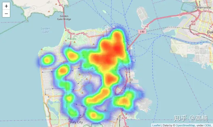
- F& s: U1 |6 G7 W8 G7 V" B 10. 创建热力图
9 L1 ^3 W6 f, E+ ^
from folium.plugins import HeatMap
( G! S% `# T x8 x! d, p6 _& t! X- s% [' g- M- \
# lets start again with a clean copy of the map of San Francisco
6 G2 j# T- i0 |5 h" `4 ^5 G san_map = folium.Map(location = [latitude, longitude], zoom_start = 12)
( D/ h, e" `, m$ t: k* T9 e
9 ?4 M+ T, S& N; b. x # Convert data format/ Y6 B0 Z7 e/ @0 ^ z- E
heatdata = data[[Y,X]].values.tolist()
8 @4 a8 C; `* |
9 ^/ E9 A+ U) B8 D4 f, y # add incidents to map. k) t4 ~. @2 _$ u" z" ]9 b( |
HeatMap(heatdata).add_to(san_map)
% N- o& _' H; N* a6 @3 c! k- S& P
- A$ A" L1 W$ y. Z- P9 _$ c san_map
0 f# k2 b: g& Y0 Q
. n Z7 Q9 o4 q3 b, X
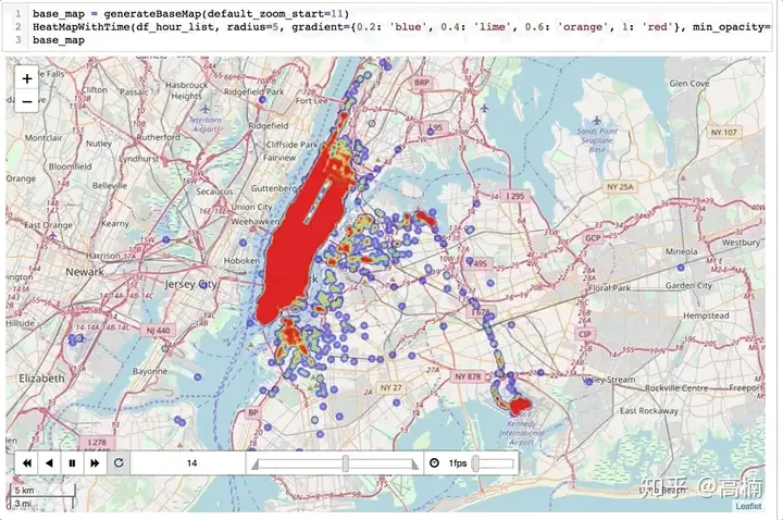
最后,folium还可以用来创建动态热力图,动态路径图等,具体可参考Medium上的这篇文章。
0 W) G4 t0 Q, N- U& H8 z) e, | 实现效果如下图所示 (直接从Medium上抱过来的图,详细代码请点击上述链接)。
) D; X! i# \* t0 S
E0 f% P, |8 T+ i# {/ u 我的其他回答:
/ N. V+ v4 s3 `
@5 w3 J* d$ E
7 I- j m9 V( E2 u2 [* R5 ]
1 L% T" H1 k N& r, ~ 最近有小伙伴私信我推荐一些学习编程的经验,我给大家几点建议:
" m1 Q l) \! T6 [, o# d W- I
1. 尽量不去看那些冗长的视频教程,不是说学不到知识,而是,在你学到知识之前,你可能已经睡着了 =_=
- x0 `( i3 E+ `6 I* } 2. 不要贪多,选一个知名度高的python教程,教学为辅,练习为主。要随时记住,我们学习python的目的在于会用,而不是背过了多少知识点。
' }- o; X& G6 Z% w1 m+ f
给大家推荐一款我超喜欢的python课程——夜曲编程。我闲没事在上面刷了一些编程题目,竟回想起当年备考雅思时被百词斩支配的恐惧。这款课程对新手小白很适合。虽然有手机app,但我建议你们用网页端学习哈。
$ C3 O3 ?& k' ~2 S) k
最后,我的终极建议是:无论选什么教程,贪多嚼不烂,好好专注一门课程,勤加练习才是提高编程水平的王道。等基础知识学的差不多了,去Kaggle上参加几场比赛,琢磨琢磨别人的编程思路和方法就完美啦!
' B* ~+ \+ y* X& z/ f' k7 J3 W/ |% n% r# p