|
3 D, E" K. B' W. v. @
原创:宋宋 Python专栏
! u% z# i6 _! s M9 N# e 来源:Python数据分析:折线图和散点图的绘制
$ `: {) c: M) n6 n 折线图 k8 B! G; _, s# ^7 O
折线图用于分析自变量和因变量之间的趋势关系,最适合用于显示随着时间而变化的连续数据,同时还可以看出数量的差异,增长情况。
% J: r& x) w# S- C: v$ L% ~* j Matplotlib 中绘制散点图的函数为 plot() ,使用语法如下: matplotlib.pyplot.plot(*args, scalex=True, scaley=True, data=None, **kwargs)1) 简单的折线图 & _3 y. _2 k5 P
在matplotlib面向对象的绘图库中,pyplot是一个方便的接口。
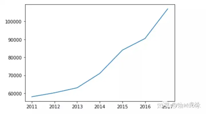
\ O! t+ k% D! E; n. p plot()函数:支持创建单条折线的折线图,也支持创建包含多条折线的复式折线图----只要在调用plot()时传入多个分别代表X轴和Y轴数据的list列表即可。 7 M. b& T7 N m) J% P( E! v
import matplotlib.pyplot as plt
9 W+ |6 U, U5 k0 _0 ~" F: L
( {! U. E: Z+ x' n x_data = [2011,2012,2013,2014,2015,2016,2017]( n/ D6 t6 e/ C3 Z9 b' h" K
y_data = [58000,60200,63000,71000,84000,90500,107000]
9 |+ ~3 n% b5 a# ^9 }$ N* V- V3 J
# N5 L' f( }. f4 f8 U$ q) i9 i, @ plt.plot(x_data,y_data)3 T3 y9 c1 ^! D M, ~" @
plt.show()
3 h8 }; h" O8 K9 y7 n6 r" c) ~6 N
! T- N! c9 q9 S! b# G# F% ]4 e6 T7 a 6 ^1 H7 W2 l) f v
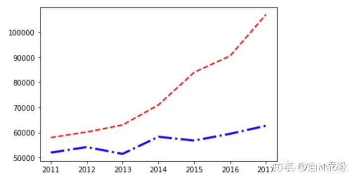
2)复式折线图:
0 _9 |3 a3 `2 }5 W8 J ?! |. [& F import matplotlib.pyplot as plt& E5 }" D' F* v% m! f6 v" W! L
x_data = [2011,2012,2013,2014,2015,2016,2017]
* L% U% Q W6 m: s s' V+ y y_data = [58000,60200,63000,71000,84000,90500,107000]. I7 Y5 a2 P1 m
y_data2 = [52000,54200,51500,58300,56800,59500,62700]
, ^7 M: _9 S' |
$ T0 D2 k' h6 e) M) @, y' q) k plt.plot(x_data,y_data,color=red,linewidth=2.0,linestyle=--)
. N' y, G/ O2 b: t1 c plt.plot(x_data,y_data2,color=blue,linewidth=3.0,linestyle=-.), ^6 j* f {+ a+ A( h3 G7 J/ G
plt.show()9 L0 {$ v; A, u0 P8 a
$ _% j7 C/ {1 h2 B1 I# ]
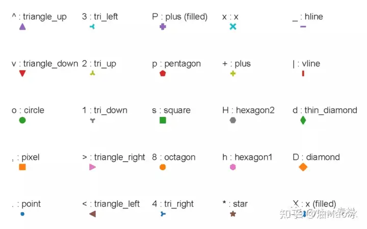
" l" M% K; d: [7 r, W% M 注:说明:参数color=’ red ‘,可以换成color=’ #054E9F’,每两个十六进制数分别代表R、G、B分量,除了使用red、blue、green等还可以参照下图小白参数linestyle可以选择使用下面的样式: - solid line style 表示实线-- dashed line style 表示虚线-. dash-dot line style 表示短线、点相间的虚线: dotted line style 表示点线参数 linewidth 可以指定折线的宽度参数 marker 是指标记点,有如下的:
( V% ~8 M5 @% l7 l+ b' l" Q+ T @! X) Q4 K5 C4 W
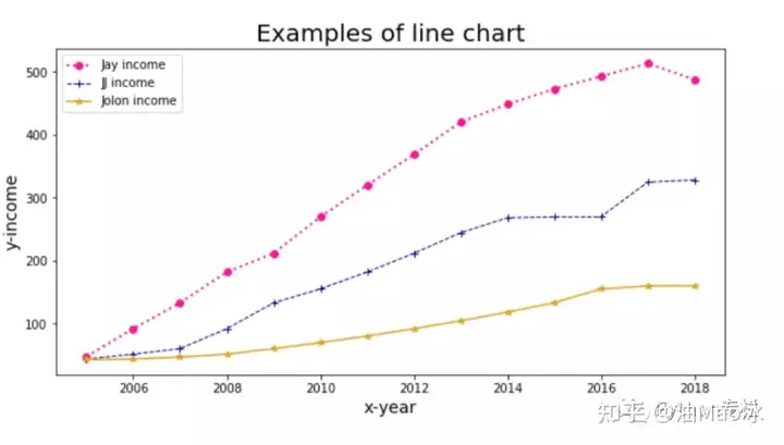
3) 管理图例 对于复式折线图,应该为每条折线添加图例,可以通过legend()函数来实现。该函数可传入两个list参数,其中第一个list参数(handles参数)用于引用折线图上的每条折线;第二个list参数(labels)代表为每条折线所添加的图例 9 G2 `/ s( v: A% w
import pandas as pd
! C! [ Z/ T7 [+ z) L import matplotlib.pyplot as plt [4 l2 j0 T! W9 q
0 x9 E6 e" d+ M8 D
#读取数据2 f" s# R3 M9 j. Z
data = pd.read_excel(matplotlib.xlsx)* `+ l* B5 H& ^3 G2 O% m7 |
0 L8 T; F: ]. w
plt.figure(figsize=(10,5))#设置画布的尺寸
( E+ v# N2 a# P$ O0 A2 b plt.title(Examples of line chart,fontsize=20)#标题,并设定字号大小
8 T- n- F0 Y5 R plt.xlabel(ux-year,fontsize=14)#设置x轴,并设定字号大小
: Q& r3 k; W5 k' u7 u; |- T8 F6 }) w plt.ylabel(uy-income,fontsize=14)#设置y轴,并设定字号大小& b# U$ K% H$ n( l0 I6 I' K
/ O' V: C5 A* ~8 y o1 P #color:颜色,linewidth:线宽,linestyle:线条类型,label:图例,marker:数据点的类型+ V$ \( ?. u, p) f+ {! q1 d
in1, = plt.plot(data[时间],data[收入_Jay],color="deeppink",linewidth=2,linestyle=:, marker=o)& B& J' d7 X$ A( d, x$ b" ^; z& a k0 M
in2, = plt.plot(data[时间],data[收入_JJ],color="darkblue",linewidth=1,linestyle=--, marker=+)9 K. l9 c; v$ |, @
in3, = plt.plot(data[时间],data[收入_Jolin],color="goldenrod",linewidth=1.5,linestyle=-, marker=*)4 n6 |: L: K' e, P+ Y
( K# J0 u8 ?, [! e# [# T- W plt.legend(handles = [in1,in2,in3],labels=[Jay income,JJ income,Jolon income],loc=2)#图例展示位置,数字代表第几象限 D* i7 k! ]1 f5 }
plt.show()#显示图像. _4 j( s# g( ]! v5 e0 B# A8 h' V
; s4 D9 H* C! ]' E' }6 W& L, c
, n$ Q. D) k- L' U4 ^
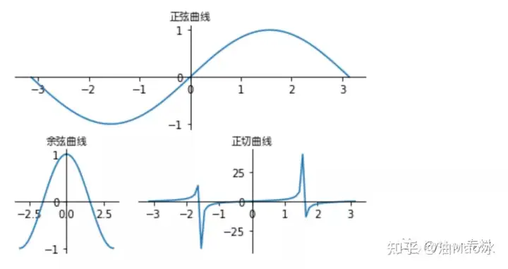
4) 管理多个子图 # X) H8 f8 k1 D% F; Y+ i
import matplotlib.pyplot as plt w1 N3 ~& x2 b7 t( ~
import numpy as np
# ?& @3 m5 w) @- z import matplotlib.gridspec as gridspec
2 n7 {; |8 l2 f! z import matplotlib.font_manager as fm #字体管理器: l' ?% p5 w2 w- k" k2 w
* o. r, h+ a. d; `: M2 N) V s my_font = fm.FontProperties(fname="/System/Library/Fonts/PingFang.ttc")
% b- w6 m5 i1 e# j ^; P3 E3 `- E- }2 U9 e
plt.figure()- y! e0 i6 D, O; c* h- U6 h
, x2 }+ o! L A( Y4 y5 u& e& m
x_data = np.linspace(-np.pi,np.pi,64,endpoint=True)
3 x9 l. V, g( B q% K& W: Y9 K gs = gridspec.GridSpec(2,3) #将绘图区分成两行三列
# z% S4 |/ ]8 V2 D' m ax1 = plt.subplot(gs[0,:])#指定ax1占用第一行(0)整行5 a3 j& A2 M) X4 S
ax2 = plt.subplot(gs[1,0])#指定ax2占用第二行(1)的第一格(第二个参数为0)! }* H: C; g& ~9 j
ax3 = plt.subplot(gs[1,1:3])#指定ax3占用第二行(1)的第二、三格(第二个参数为1:3)
1 f# p$ w2 s G& g3 U D& p& ?' u/ M+ h- P) M8 D- L
#绘制正弦曲线
8 Z" r f5 z* b) ~7 i S- J& R: M ax1.plot(x_data,np.sin(x_data))) u) z$ f; Q, f) J7 f( _
ax1.spines[right].set_color(none)
, t3 @9 v! S7 S2 r: I ax1.spines[top].set_color(none)& O+ u0 _; u6 j3 `: ?6 h
ax1.spines[bottom].set_position((data,0))
) y; R: r2 Q1 k( a. S( |2 M ax1.spines[left].set_position((data,0)). w* M* K' S6 Y6 z0 M* k; G
ax1.set_title(正弦曲线,fontproperties=my_font)
7 q; ?; [0 S$ ~* z- w0 C L& `* ^
#绘制余弦曲线- O3 B* n. e# g0 D; B
ax2.plot(x_data,np.cos(x_data))
% j6 q' v' t+ m4 p ax2.spines[right].set_color(none)
4 H( ^6 p5 s* C4 G# B ax2.spines[top].set_color(none)8 y- u5 P1 P8 i3 K1 e2 ?+ ?
ax2.spines[bottom].set_position((data,0))
6 n9 W% e, y/ |, _9 o2 L ax2.spines[left].set_position((data,0))# Z( D! `9 \& r+ e" s4 B. d
ax2.set_title(余弦曲线,fontproperties=my_font)
3 X2 \. x& p9 L. R6 g+ U& _ g+ O- r
* S% z9 q* x9 f7 ^- X8 a8 _ #绘制正切曲线+ _9 q, z+ f% g7 S; Y. O0 }
ax3.plot(x_data,np.tan(x_data))
" [6 H4 |& U+ }7 P ax3.spines[right].set_color(none)
( \/ }. T7 c* `5 I ax3.spines[top].set_color(none): c: ~5 j f/ [# l; X' G4 G
ax3.spines[bottom].set_position((data,0))0 m" d, h( ^. v9 ~# T
ax3.spines[left].set_position((data,0))
4 N& s$ {1 L. V- r ax3.set_title(正切曲线,fontproperties=my_font)% y- N+ X8 {& O( F4 q2 h" |
plt.show()
" g9 r+ I1 z% A0 O
; ^0 M2 c* f% X r" W7 \3 j2 ?, t6 r 结果:
# Y& k& f6 _1 o4 k! K* [! r
" O, I- L/ k# G4 }
3 ^# w' M2 Z+ ^% N0 l
, b) {9 J/ b. L+ s& t) A" a' C5 n$ d* z+ b- a! c
2 {' Z3 n) L w( `1 t
: g$ r7 Z0 @0 U6 z+ U |